
Inspiration
I first came across satellite imagery as a data source through its use in estimating oil inventories. Analysts could use the shadows inside storage tanks with floating roofs to work out roughly how much oil they held.
This gave me the idea on testing whether free satellite imagery could give an independent view of ship activity through the Strait of Hormuz, where AIS-based tracking depends on the signals ships transmit.
Detection windows
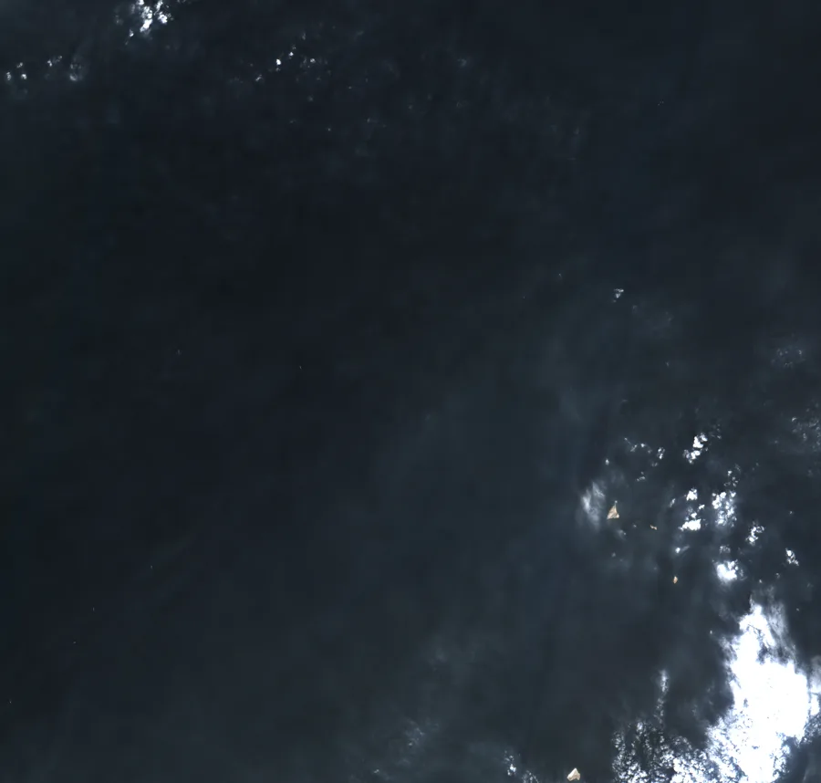
The Python scripts query the Planetary Computer STAC catalogue, make previews and extract candidate detections. The optical script also saves 80×80-pixel crops around up to six of the largest detections and enlarges them for viewing for comparison and manual validation.
Clouded judgement
Before looking for ships, the optical script uses Sentinel-2’s Scene Classification Layer (SCL) to exclude likely clouds and cloud shadows, and expands the excluded areas around their edges. The SCL isn't 100% accurate, and several small clouds still reached the detector, which picked them up because they were bright against the surrounding water and shows the need for better detection rules or models.
The fourth and fifth cutouts show ships, while the others show clouds. Shape, wakes and the colour offset between optical bands offered possible ways to distinguish them, but there was no implemented second-stage classifier to make that distinction automatically, so the initial bright-object count was still too crude to use as a traffic series.
A change of port
Unfortunately the Strait of Hormuz didn't have a lot of shipping traffic during this period as one would expect, which posed a problem for our research problem. I considered using PortWatch as an additional means to track ship positions to compare with our sparse data, but PortWatch was rate-limiting our requests, and its reliance on AIS raised another issue. Missing transmissions and interference around Hormuz meant I couldn’t simply treat the reported traffic as a complete record.
I shifted to Singapore’s anchorages to work on the narrower, simpler problem of ship detection and to test the limits of free satellite data in a far simpler context. The charted boundaries gave me defined areas where I could compare radar detections with manual counts before testing whether those counts were useful for predicting bunker fuel sales.
Drawing the line
The satellite view below puts the Singapore study in context. Ships are visible off the southern and eastern coast, around the port and its anchorages. These are the waters I focused on for the counting exercise, using radar imagery for the detections and this optical view to show the geography.
The counting areas came from MPA’s anchorage chartlet, whose PDF drawing outlines were converted into geographic coordinates and checked against the map’s coordinate ticks, the satellite coastline and the visible arrangement of anchored ships. I grouped the areas into bunkering, petroleum and general anchorages, with small-craft, quarantine and special-purpose zones excluded, and added a separate waiting-area box east of the port limits. Six chartlet boundaries needed reconstruction, and that eastern box was drawn manually, so the dashed outlines mark approximate areas rather than precise official boundaries.
Identifying ships
For Singapore I used Sentinel-1 radar, which avoids the optical cloud problem but still needs to distinguish ships from the surrounding sea. The CFAR detector compares a bright candidate with a ring of nearby water, leaving a guard area around the candidate so the ship itself does not dominate that comparison. A fixed brightness threshold had been unreliable across different water backgrounds, while comparing locally gave the threshold a reference for each part of the scene.
- Radar passesSelect images covering the Singapore anchorages.
- Local detectionUse CFAR within the anchorage polygons.
- Coverage adjustmentAggregate to average ships per pass.
- Forecast comparisonCompare bunker-sales predictions with a past-data baseline.
Looking at the outputs also exposed counting problems. A large tanker could appear as separate bright bow and stern pieces, so the detector grows connected bright pixels and the analysis merges detections within 150 metres. Land is masked with a buffer around the coast, and smaller radar fragments are kept out of the main count. Those changes address specific failure cases; they do not turn every remaining box into a verified ship.
The saved hand check covers ten zone crops on seven dates, with 113 ships counted by the detector and 113 by eye in total, and no crop differing by more than one. That is a useful initial check, but equal totals can hide misses and false positives, crowded nearshore scenes remain difficult to judge, and the large eastern waiting area was not hand-counted. It supports inspecting the measurement before using it, rather than claiming a general detection accuracy from a small sample.
Mapping it out
The Singapore pipeline covers 830-plus radar passes, using a CFAR detector within anchorage boundaries derived from MPA’s chartlet. Coverage varied from two to nine passes a month, so we used average ships per pass to account for the differing frequencies (monthly sums would be inaccurate).
The prediction target was monthly bunker fuel sold, and the estimate was made after the month ended but before MPA’s assumed release date on the tenth of the following month. The original historical-sales model started from the previous month’s sales and used the same monthly change one year earlier; the satellite version added the current month’s change in average orbit-adjusted ships per pass. Both were refitted on earlier months only, and the comparison used the same 82 eligible months from January 2019 to September 2026, with gaps where the primary satellite feature was unavailable.
The original combined model’s mean absolute percentage error was 4.70%, compared with 4.68% using historical sales alone, so adding the total ship count did not improve that test. A petroleum-anchorage subgroup looked better after comparing several groups, which made it a research lead rather than the original result. The sales labels are revised official figures, and the archived image dates do not recreate every piece of first-release information a live forecaster would have had.
Standalone prediction
I also tested whether satellite counts could estimate monthly sales on their own. This model learns the relationship between ship counts and sales from earlier months, then uses the current month’s average orbit-adjusted ship count to estimate the sales level. It has no previous-month sales or seasonal sales input when making that estimate.
The standalone model reached 6.69% MAPE on those same 82 months, while simply carrying the previous month’s sales forward gave 5.31%. Its estimates stayed near a typical sales level and missed both monthly spikes and the higher level of demand in the later years. Historical sales were training labels for this model, but previous sales were not an input when making its estimate, so it really did have to make do with the satellite count.
That result made the measurement mismatch worth looking at directly. The satellite feature is average occupancy at a few observation times, while bunker sales are fuel delivered across a whole month. The number of visits, how long ships stay, how much fuel each buys and activity outside the counted anchorages can all change without a proportional change in visible ships, although those mechanisms would need their own data before I could attribute the errors to them.
Moving together
There were stretches where counts and sales looked promising together, so I compared monthly percentage changes and checked whether the relationship depended on the time window or a delay between the two series. The same-month change correlation was −0.09 across the 82 evaluation months, and both moved in the same direction in 45.1% of them. Dividing sales by the days in each month reduced the variance of sales changes by about 42.5%, but the correlation with count changes was still only +0.03, so calendar duration explained part of the sales variation without revealing a strong positive link to the counts.
The relationship did change over time. The trailing 12-month correlation reached +0.53 in February 2021, but fell to −0.69 in October 2022. The 24-month check also changed sign. There were periods of positive co-movement, though the pattern was unstable rather than a consistently positive link.
I also compared ship-count changes with sales changes up to three months earlier and later. When ships led sales by one month, the correlation was weakly positive at +0.15; leads of two and three months were near zero. Using the same 52 observations at every offset left the one-month lead small at +0.13. These are exploratory checks on data already examined, rather than evidence that a revised model would forecast better.
Taking a step back
In February 2022, fuel sales fell 13% while our ship count increased. January had 31 days and February had 28, so even with the same daily fuel sales, February’s monthly total would be about 9.7% lower. After accounting for the number of days, daily sales fell only 3.6%. Argus also reported that other Asian ports were offering more competitive prices, so there were reasons for fuel purchases to change even if ships were still present in Singapore.
December 2023 exposed a different limitation. Sales increased about 18% while our count fell, and the EIA linked the higher demand around this period to longer voyages avoiding the Red Sea. That gives us a plausible reason for the two series to diverge: ships could buy more fuel per visit without more ships appearing in an image. We hadn’t measured purchases per ship, so we couldn’t test that explanation directly, and counting the ships more accurately would not necessarily have supplied the missing information.
The largest miss came in December 2025, when the satellite-only estimate was 24% too low. Sales rose sharply while the count barely changed, and we haven’t established what drove that increase. One possibility is precautionary fuel buying amid renewed threats of conflict with Iran, although the 29 December warning came late in the month and we haven’t established a link to purchases. The result shows where the count failed to capture demand, but explaining the spike would require information about the vessels, their fuel purchases and the market conditions that month.
A fairer comparison
I then tested a fixed group of repairs against the problems the diagnostics had exposed. Sales were converted to tonnes per day and reconstructed using the known length of the target month, and the history models were given the previous month’s sales growth alongside the seasonal change. I compared expanding history with a trailing five-year window, then tried current counts, counts one month earlier, a three-month count average, petroleum-anchorage counts and a radar size proxy. The last proxy gives larger retained radar footprints more weight, but it measures bright radar response rather than actual hull area or fuel capacity.
The biggest improvement came from the forecasting setup. MAPE fell from the original history model’s 4.68% to 4.14% with daily-sales seasonal modelling, and to 3.90% when previous-month growth was also included. Shortening the history alone did not improve the daily seasonal model, and the five-year version with previous growth reached 3.94%, slightly behind the expanding version. That matters because an improved model containing satellite data would otherwise make it easy to credit the images for gains that came from the baseline.
For each satellite addition I also fitted a history-only control on exactly the same earlier months, because missing satellite observations can otherwise change the training sample as well as the inputs. Total counts gave 3.94% MAPE against their matched control’s 3.91%, so they still did not help. Petroleum counts reached 3.74% against a 3.93% control, an improvement of about 0.19 percentage points, while smoothing and size weighting gave much smaller changes. The lagged-count candidate needed four history-only fallbacks when its input was missing, and every evaluation month remained in the comparison.
A recalibrated standalone count model with calendar adjustment and a recent three-year training window improved on the first standalone attempt, but its 5.11% error was barely better than the matched recent-mean control’s 5.16% and remained worse than the revised history models. The petroleum result is the stronger lead, although the group had already been inspected and the error comparisons helped select it, so the apparent gain still needs evidence beyond these historical months.
Further comparison
Before retrieving October 2026’s official sales figure, I froze predictions from the revised models using the existing September sales history and October satellite inputs. The retrieved figure was 5.315 million tonnes, and the revised expanding-history model estimated 4.850 million, an 8.75% underestimate, compared with 10.50% for the original history model and 21.45% for the original satellite-only model.
The petroleum candidate estimated 4.831 million tonnes, missing by 9.10%, while its matched history control missed by 8.79%. This single additional historical month is too small to validate a model, but it is a useful check against the temptation to stop at the best development score: the better baseline carried over in that month, and the selected satellite addition did not.
Better data
There are two directions I would pursue from here, because the weak relationship could reflect both what the images miss and what a ship count leaves out about fuel demand. More frequent observations could help estimate arrivals, departures, turnover and time spent at anchor, while higher-resolution imagery could improve detection and support estimates of vessel size. Linking those observations to AIS records or vessel registries could also help distinguish ship types and capacities, so the feature could describe the activity taking place rather than just how many bright objects were present.
That would still need validation against independently identified ships, and even a correctly identified vessel’s capacity would not tell me how much fuel it purchased on that visit. Fuel deliveries would usually need transaction or operational records, while a useful estimate of turnover would need observations frequent enough to distinguish ships arriving and leaving between images. These are proposed measurement improvements; the limited hand checks so far do not establish that inaccurate detection caused the forecasting errors.
Understanding the trade
The other direction is to understand the bunkering process well enough to decide which observations should matter. A ship can be at anchor for reasons other than refuelling, and a fuel purchase depends on more than its presence: the voyage ahead, fuel remaining onboard, the quantity it can take, the services being arranged and the commercial choices around the stop could all be relevant. I would want to understand who makes that decision, whether onboard or through the owner, charterer or a purchasing team, and what information they use.
Pricing would be part of that investigation, including whether Singapore is attractive relative to other refuelling ports, whether contracts affect where fuel is bought and how availability or delivery time changes the quantity ordered. Those mechanisms have not been measured in this study, so they are questions for domain research rather than explanations I can assign to every error. Better imagery would help describe the activity, and understanding the purchase decision would help choose which parts of that activity are worth using to predict fuel sales volume.
Final thoughts
The useful outcome so far is a better specified prediction problem and a stronger historical baseline, alongside a narrower satellite hypothesis. The count still covers only a few snapshots each month and only selected anchorages, the radar size proxy is not measured vessel capacity, and the historical tests use revised official sales. There is no demonstrated general satellite advantage or validated explanation for every demand spike.
The next check is to freeze the revised expanding-history model, the five-year matched history control and its petroleum-count addition, then collect a consecutive run of new months without changing the features after seeing each result. The plan records the first retrieved official figure and the image cutoff for each issue, keeps misses visible and compares the paired errors over the full sequence. More hand-labelled detections and data on vessel size, turnover and actual fuel purchases would address different parts of the measurement problem, but adding them would need a separate declared experiment.